Week 2 - Image Preprocessing

Hello everyone, welcome to my blog again. It has been a busy week for me, and I did some work to preprocess the images for recognition.

See my work!

In order to give you a clearer idea of what I did, I put some extra efforts to put my work as an web app using the free hosting service Heroku (huge thanks to them!), so that you can get your hands on and experiment with the program I wrote. You may find it here: https://senior-project.jessexu.me/?file_selection=Week+2 (loading time may be a bit long because the images are being processed in real-time, and make sure you have good Internet)

What does the program do?

You may be a bit confused if you head straight into the web app above, so let me explain what is the program I wrote this week doing.

I will use the parameters that I set as the default of the app when I’m explaining. They turn out to produce pretty good results after I experimented with them.

Default parameters

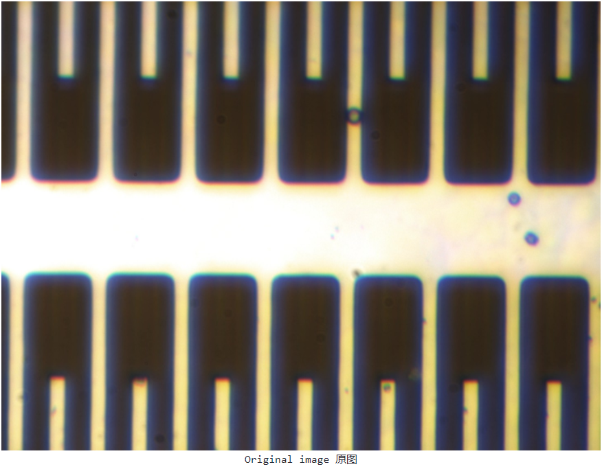
Let’s start with the original image. It’s a photo of a part of the gyroscope. As mentioned in last week’s blog post, the preprocessing I need to apply on the photo is to denoise the image, find the contours of the part (in this photo’s case, the contours of the broaches/combs), and find the corners of the parts.

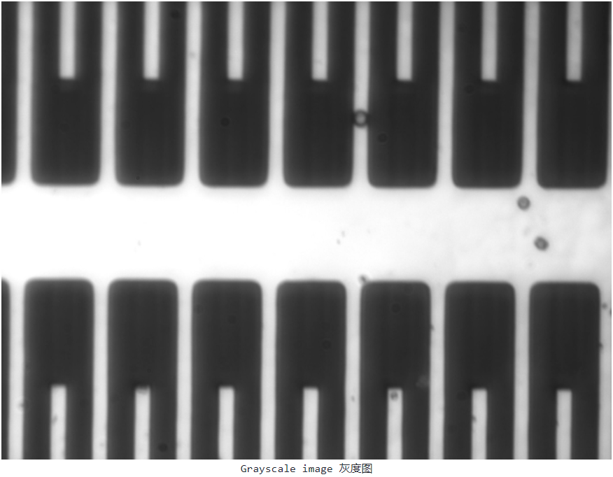
First, we need to turn it into a grayscale image for further processing. OpenCV has a handy method for this:

gray = cv2.cvtColor(img, cv2.COLOR_BGR2GRAY)

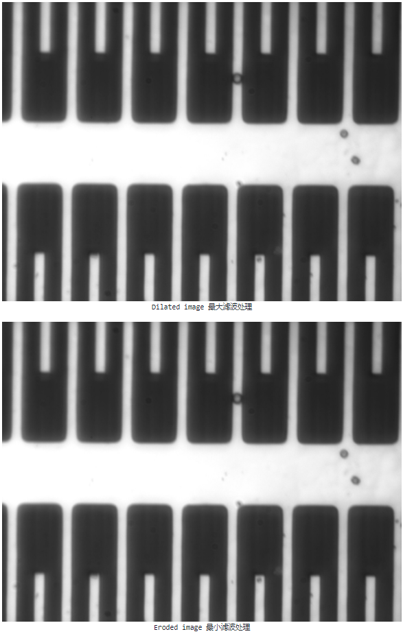
Then, we can filter out some of the noise in the photo to get a clearer shot by first dilating then eroding the image. It can be done with the following two lines of code. With higher iterations, more noise will be filtered out, but it may also distort the image.

kernel = np.ones((3, 3), np.uint8) # We use a commonly used 3x3 kernel for this.
dilated_img = cv2.dilate(gray, kernel, iterations) # gray is the grayscale image.
eroded_img = cv2.erode(dilate_img, kernel, iterations)

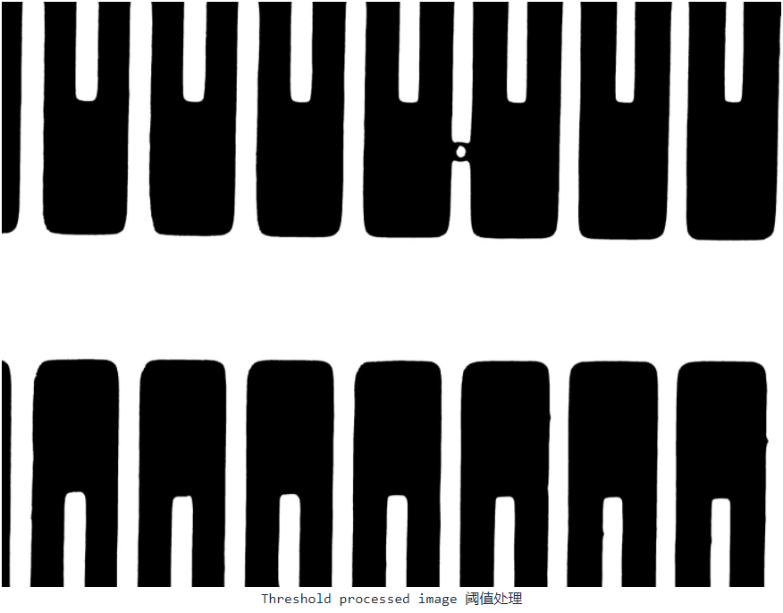
Then, we can apply a threshold to the image with the following code to get a binary image from the de-noised image. You can see that one of the dirty points that did not get removed from previous processes was retained in the threshold processed image.

cv2.threshold(erosion, threshold_value, 255, cv2.THRESH_BINARY)

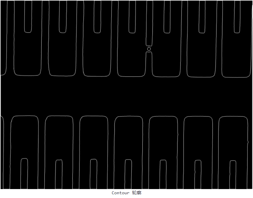
With the binary image we have, we can get the contour of the shapes with the code below and draw it out. As you can see, the contours are quite clear.

contours, hierarchy = cv2.findContours(binary_image, cv2.RETR_TREE, cv2.CHAIN_APPROX_SIMPLE)

Lastly, we run a Hough Line Transform to detect the lines in the contours image, so we can find the corners and dimensions of the shapes. The code used here is

lines = cv2.HoughLinesP(img, 1, np.pi/180, 100,minLineLength=100, maxLineGap=10)

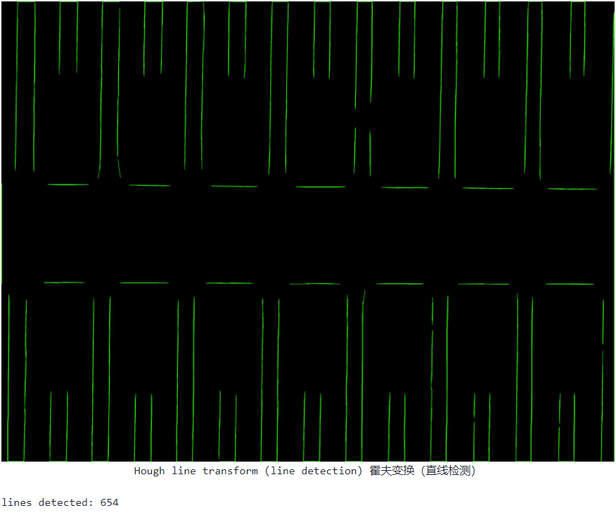
However, the results I get here is not very impressive, as it detects way more lines than it should, and there are small line segments clustered together if you zoom in the image. So, I will focus on fine-tuning the parameters for the Hough Line Transform next week.